targets::tar_script()13 Build automation with targets
We are finally ready to actually build a pipeline. For this, we are going to be using a package called {targets} (Landau 2021) which is a so-called “build automation tool”.
If you go back to the reproducibility iceberg, you will see that we are quite low now.
Without a build automation tool, a pipeline is nothing but a series of scripts that get called one after the other, or perhaps the pipeline is only one very long script that does the required operations successfully.
There are several problems with this approach, so let’s see how build automation can help us.
13.1 Introduction
Script-based workflows are problematic for several reasons. The first is that scripts can, and will, be executed out of order. You can mitigate some of the problems this can create by using pure functions, but you still need to make sure not to run the scripts out of order. But what does that actually mean? Well, suppose that you changed a function, and only want to re-execute the parts of the pipeline that are impacted by that change. But this supposes that you can know, in your head, which part of the script was impacted and which was not. And this can be quite difficult to figure out, especially when the pipeline is huge. So you will run certain parts of the script, and not others, in the hope that you don’t need to re-run everything.
Another issue is that pipelines written as scripts are usually quite difficult to read and understand. To mitigate this, what you’d typically do is write a lot of comments. But here again you face the problem of needing to maintain these comments, and once the comments and the code are out of synch… the problems start (or rather, they continue).
Running the different parts of the pipeline in parallel is also very complicated if your pipeline is defined as script. You would need to break the script into independent parts (and make really sure that these parts are independent) and execute them in parallel, perhaps using a separate R session for each script. The good news is that if you followed the advice from this book you have been using functional programming and so your pipeline is a series of pure function calls, which simplifies running the pipeline in parallel.
But by now you should know that software engineers also faced similar problems when they needed to build their software, and you should also suspect that they likely came up with something to alleviate these issues. Enter build automation tools.
When using a build automation tool, what you end up doing is writing down a recipe that defines how the source code should be “cooked” into the software (or in our case, a report, a cleaned dataset or any data product).
The build automation tool then tracks:
- any change in any of the code. Only the outputs that are affected by the changes you did will be re-computed (and their dependencies as well);
- any change in any of the tracked files. For example, if a file gets updated daily, you can track this file and the build automation tool will only execute the parts of the pipeline affected by this update;
- which parts of the pipeline can safely run in parallel (with the option to thus run the pipeline on multiple CPU cores).
Just like many of the other tools that we have encountered in this book, what build automation tools do is allow you to not have to rely on your brain. You write down the recipe once, and then you can focus again on just the code of your actual project. You shouldn’t have to think about the pipeline itself, nor think about how to best run it. Let your computer figure that out for you, it’s much better at such tasks than you.
13.2 {targets} quick-start
First thing’s first: to know everything about the {targets} package, you should read the excellent {targets} manual1. Everything’s in there. So what I’m going to do is really just give you a very quick intro to what I think are really the main points you should know about to get started.
Let’s start with a “hello-world” type pipeline. Create a new folder called something like targets_intro/, and start a fresh R session in it. For now, let’s ignore {renv}. We will see how {renv} works together with {targets} to provide an (almost reproducible) pipeline later. In that fresh session inside the targets_intro/ run the following line:
this will create a template _targets.R file in that directory. This is the file in which we will define our pipeline. Open it in your favourite editor. A _targets.R pipeline is roughly divided into three parts:
- first is where packages are loaded and helper functions are defined;
- second is where pipeline-specific options are defined;
- third is the pipeline itself, defined as a series of targets.
Let’s go through all these parts one by one.
13.2.1 _targets.R’s anatomy
The first part of the pipeline is where packages and helper functions get loaded. In the template, the very first line is a library(targets) call followed by a function definition. There are two important things here that you need to understand.
If your pipeline needs, say, the {dplyr} package to run, you could write library(dplyr) right after the library(targets) call. However, it is best to actually do as in the template, and load the packages using tar_option_set(packages = "dplyr"). This is because if you execute the pipeline in parallel, you need to make sure that all the packages are available to all the workers (typically, one worker per CPU core). If you load the packages at the top of the _targets.R script, the packages will be available for the original session that called library(...), but not to any worker sessions spawned for parallel execution.
So, the idea is that at the very top of your script, you only load the {targets} library and other packages that are required for running the pipeline itself (as we shall see in coming sections). But packages that are required by functions that are running inside the pipeline should ideally be loaded as in the template. Another way of saying this: at the top of the script, think “pipeline infrastructure” packages ({targets} and some others), but inside tar_option_set() think “functions that run inside the pipeline” packages.
Part two is where you set some global options for the pipeline. As discussed previously, this is where you should load packages that are required by the functions that are called inside the pipeline. I won’t list all the options here, because I would simply be repeating what’s in the documentation2. This second part is also where you can define some functions that you might need for running the pipeline. For example, you might need to define a function to load and clean some data: this is where you would do so. We have developed a package, so we do not need such a function, we will simply load the data from the package directly. But sometimes your analysis doesn’t require you to write any custom functions, or maybe just a few, and perhaps you don’t see the benefit of building a package just for one or two functions. So instead, you have two other options: you either define them directly inside the _targets.R script, like in the template, or you create a functions/ folder next to the _targets.R script, and put your functions there. It’s up to you, but I prefer this second option. In the example script, the following function is defined:
summarize_data <- function(dataset) {
  colMeans(dataset)
}
Finally, comes the pipeline itself. Let’s take a closer look at it:
list(
  tar_target(data,
             data.frame(x = sample.int(100),
                        y = sample.int(100))),

  tar_target(data_summary,
             summarize_data(data)) # Call your custom functions.
)
The pipeline is nothing but a list (told you lists were a very important object) of targets. A target is defined using the tar_target() function and has at least two inputs: the first is the name of the target (without quotes) and the second is the function that generates the target. So a target defined as tar_target(y, f(x)) can be understood as y <- f(x). The next target can use the output of the previous target as an input, so you could have something like tar_target(z, f(y)) (just like in the template).
13.3 A pipeline is a composition of pure functions
You can run this pipeline by typing tar_make() in a console:
targets::tar_make()• start target data
• built target data [0.82 seconds]
• start target data_summary
• built target data_summary [0.02 seconds]
• end pipeline [1.71 seconds]The pipeline is done running! So, now what? This pipeline simply built some summary statistics, but where are they? Typing data_summary in the console to try to inspect this output results in the following:
data_summaryError: object 'data_summary' not foundWhat is going on?
First, you need to remember our chapter on functional programming. We want our pipeline to be a sequence of pure functions. This means that our pipeline running successfully should not depend on anything in the global environment (apart from loading the packages in the first part of the script, and the options set with tar_option_set() for the others) and it should not change anything outside of its scope. This means that the pipeline should not change anything in the global environment either. This is exactly how a {targets} pipeline operates. A pipeline defined using {targets} will be pure and so the output of the pipeline will not be saved in the global environment. Now, strictly speaking, the pipeline is not exactly pure. Check the folder that contains the _targets.R script. There should now be a _targets/ folder in there as well. If you go inside that folder, and then open the objects/ folder, you should see two objects, data and data_summary. These are the outputs of our pipeline.
So each target that is defined inside the pipeline gets saved there in the .rds format. This is an R-specific format that you can use to save any type of object. It doesn’t matter what it is: a simple data frame, a fitted model, a ggplot, whatever, you can write any R object to disk in this format using the saveRDS() function, and then read it back into another R session using readRDS(). {targets} makes use of these two functions to save every target computed by your pipeline, and simply retrieves them from the _targets/ folder instead of recomputing them. Keep this in mind if you use Git to version the code of your pipeline (which you are doing of course), and add the _targets/ folder to the .gitignore (unless you really want to also version it, but it shouldn’t be necessary).
So because the pipeline is pure, and none of its outputs get saved into the global environment, calling data_summary results in the error above. So to retrieve the outputs you should use tar_read() or tar_load(). The difference is that tar_read() simply reads the output and shows it in the console but tar_load() reads and saves the object into the global environment. So to retrieve our data_summary object let’s use tar_load(data_summary):
tar_load(data_summary)Now, typing data_summary shows the computed output:
data_summary x y
50.5 50.5It is possible to load all the outputs using tar_load_everything() so that you don’t need to load each output one by one.
Before continuing with more {targets} features, I want to really stress the fact that the pipeline is the composition of pure functions. So functions that only have a side-effect will be difficult to handle. Examples of such functions are functions that read data, or that print something to the screen. For example, plotting in base R consists of a series of calls to functions with side-effects. If you open an R console and type plot(mtcars), you will see a plot. But the function plot() does not create any output. It just prints a picture on your screen, which is a side-effect. To convince yourself that plot() does not create any output and only has a side-effect, try to save the output of plot() in a variable:
a <- plot(mtcars)doing this will show the plot, but if you then call a, the plot will not appear, and instead you will get NULL:
aNULLThis is also why saving plots in R is awkward, it’s because there’s no object to actually save!
So because plot() is not a pure function, if you try to use it in a {targets} pipeline, you will get NULL as well when loading the target that should be holding the plot. To see this, change the list of targets like this:
list(
  tar_target(data,
             data.frame(x = sample.int(100),
                        y = sample.int(100))),

  tar_target(data_summary,
             summarize_data(data)), # Call your custom functions.

  tar_target(
    data_plot,
    plot(data)
  )
)
I’ve simply added a new target using tar_target() at the end, to generate a plot. Run the pipeline again using tar_make() and then type tar_load(data_plot) to load the data_plot target. But typing data_plot only shows NULL and not the plot!
There are several workarounds for this. The first is to use ggplot() instead. This is because the output of ggplot() is an object of type ggplot. You can do something like a <- ggplot() + etc... and then type a to see the plot. Doing str(a) also shows the underlying list holding the structure of the plot, as a list.
The second workaround is to save the plot to disk. For this, you need to write a new function, for example:
save_plot <- function(filename, ...){

  png(filename = filename)
  plot(...)
  dev.off()

}
If you put this in the _targets.R script, before defining the list of tar_target objects, you could use this instead of plot() in the last target:
summarize_data <- function(dataset) {
  colMeans(dataset)
}

save_plot <- function(filename, ...){
  png(filename = filename)
  plot(...)
  dev.off()

  filename
}

# Set target-specific options such as packages.
tar_option_set(packages = "dplyr")

# End this file with a list of target objects.
list(
  tar_target(data,
             data.frame(x = sample.int(100),
                        y = sample.int(100))),

  tar_target(data_summary,
             summarize_data(data)), # Call your custom functions.

  tar_target(
    data_plot,
    save_plot(
      filename = "my_plot.png",
      data),
    format = "file")
)
After running this pipeline you should see a file called my_plot.png in the folder of your pipeline. If you type tar_load(data_plot), and then data_plot you will see that this target returns the filename argument of save_plot(). This is because a target needs to return something, and in the case of functions that save a file to disk returning the path where the file gets saved is recommended. This is because if I then need to use this file in another target, I could do tar_target(x, f(data_plot)). Because the data_plot target returns a path, I can write f() in such a way that it knows how to handle this path. If instead I write tar_target(x, f("path/to/my_plot.png")), then {targets} would have no way of knowing that the target x depends on the target data_plot. The dependency between these two targets would break. Hence why the first option is preferable.
Finally, you will have noticed that the last target also has the option format = "file". This will be topic of the next section.
It is worth noting that the {ggplot2} package includes a function to save ggplot objects to disk called ggplot2::ggsave(). So you could define two targets, one to compute the ggplot object itself, and another to generate a .png image of that ggplot object.
13.4 Handling files
In this section, we will learn how {targets} handles files. First, run the following lines in the folder that contains the _targets.R script that we’ve been using up until now:
data(mtcars)

write.csv(mtcars,
          "mtcars.csv",
          row.names = F)
This will create the file "mtcars.csv" in that folder. We are going to use this in our pipeline.
Write the pipeline like this:
list(
  tar_target(
    data_mtcars,
    read.csv("mtcars.csv")
  ),

  tar_target(
    summary_mtcars,
    summary(data_mtcars)
  ),

  tar_target(
    plot_mtcars,
    save_plot(
      filename = "mtcars_plot.png",
      data_mtcars),
    format = "file")
)
You can now run the pipeline and will get a plot at the end. The problem however, is that the input file "mtcars.csv" is not being tracked for changes. Try to change the file, for example by running this line in the console:
write.csv(head(mtcars), "mtcars.csv", row.names = F)If you try to run the pipeline again, our changes to the data are ignored:
✔ skip target data_mtcars
✔ skip target plot_mtcars
✔ skip target summary_mtcars
✔ skip pipeline [0.1 seconds]
As you can see, because {targets} is not tracking the changes in the mtcars.csv file, from its point of view nothing changed. And thus the pipeline gets skipped because according to {targets}, it is up-to-date.
Let’s change the csv back:
write.csv(mtcars, "mtcars.csv", row.names = F)and change the first target such that the file gets tracked. Remember that targets need to be pure functions and return something. So we are going to change the first target to simply return the path to the file, and use the format = "file" option in tar_target():
path_data <- function(path){
  path
}

list(
  tar_target(
    path_data_mtcars,
    path_data("mtcars.csv"),
    format = "file"
  ),
  tar_target(
    data_mtcars,
    read.csv(path_data_mtcars)
  ),
  tar_target(
    summary_mtcars,
    summary(data_mtcars)
  ),
  tar_target(
    plot_mtcars,
    save_plot(filename = "mtcars_plot.png",
              data_mtcars),
    format = "file")
)
To drive the point home, I use a function called path_data() which takes a path as an input and simply returns it. This is totally superfluous, and you could define the target like this instead:
tar_target(
  path_data_mtcars,
  "mtcars.csv",
  format = "file"
)
This would have exactly the same effect as using the path_data() function.
So now we got a target called path_data_mtcars that returns nothing but the path to the data. But because we’ve used the format = "file" option, {targets} now knows that this is a file that must be tracked. So any change on this file will be correctly recognised and any target that depends on this input file will be marked as being out-of-date. The other targets are exactly the same.
Run the pipeline now using tar_make(). Now, change the input file again:
write.csv(head(mtcars),
          "mtcars.csv",
          row.names = F)
Now, run the pipeline again using tar_make(): this time you should see that {targets} correctly identified the change and runs the pipeline again accordingly!
13.5 The dependency graph
As you’ve seen in the previous section (and as I told you in the introduction) {targets} keeps track of changes in files, but also in the functions that you use. Any change to the code of any of these functions will result in {targets} identifying which targets are now out-of-date and which should be re-computed (alongside any other target that depends on them). It is possible to visualise this using tar_visnetwork(). This opens an interactive network graph in your web browser that looks like this:
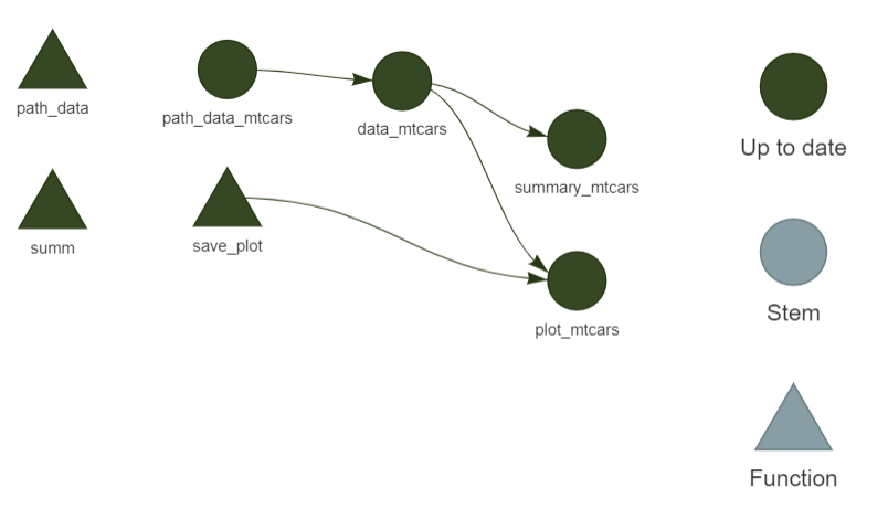
In the image above, each target has been computed, so they are all up-to-date. If you now change the input data, here is what you will see instead:
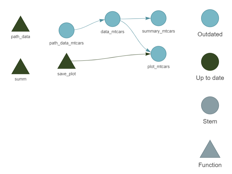
Because all the targets depend on the input data, we need to re-run everything. Let’s run the pipeline again to update all the targets using tar_make() before continuing.
Now let’s add another target to our pipeline, one that does not depend on the input data. Then, we will modify the input data again, and call tar_visnetwork() again. Change the pipeline like so:
list(
  tar_target(
    path_data_mtcars,
    "mtcars.csv",
    format = "file"
  ),
  tar_target(
    data_iris,
    data("iris")
  ),
  tar_target(
    summary_iris,
    summary(data_iris)
  ),
  tar_target(
    data_mtcars,
    read.csv(path_data_mtcars)
  ),
  tar_target(
    summary_mtcars,
    summary(data_mtcars)
  ),
  tar_target(
    plot_mtcars,
    save_plot(
      filename = "mtcars_plot.png",
      data_mtcars),
    format = "file")
)
Before running the pipeline, we can call tar_visnetwork() again to see the entire workflow:
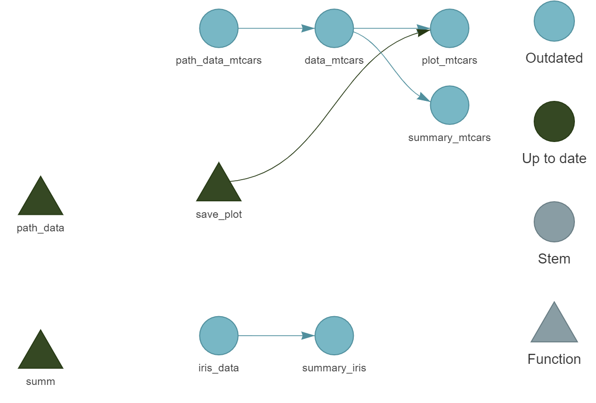
We can see that there are now two independent parts, as well as two unused functions, path_data() and summ() which we could remove.
Running the pipeline using tar_make() builds everything successfully. Let’s add the following target, just before the very last one:
tar_target(
list_summaries,
list(
"summary_iris" = summary_iris,
"summary_mtcars" = summary_mtcars
)
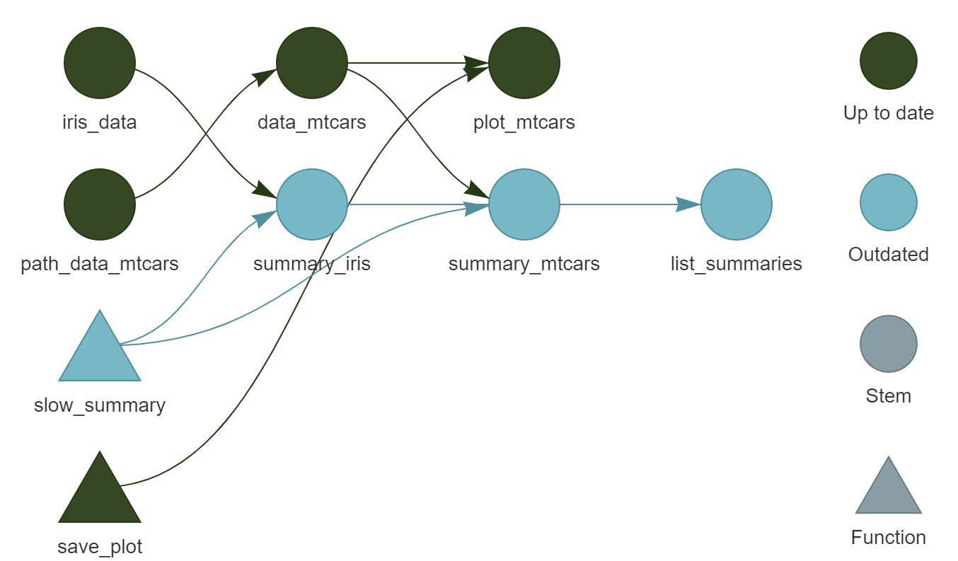
),This target creates a list with the two summaries that we compute. Call tar_visnetwork() again:
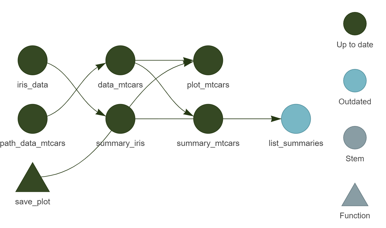
Finally, run the pipeline one last time to compute the final output.
13.6 Running the pipeline in parallel
{targets} makes it easy to run independent parts of our pipeline in parallel. In the example from before, it was quite obvious to know which parts were independent, but when the pipeline grows in complexity, it can be very difficult to see which parts are independent.
Let’s now run the example from before in parallel. But first, we need to create a function that takes some time to run. summary() is so quick that running both of its calls in parallel is not worth it (and would actually even run slower, I’ll explain why at the end). Let’s define a new function called slow_summary():
slow_summary <- function(...){
  Sys.sleep(30)
  summary(...)
}
and replace every call to summary() with slow_summary() in the pipeline:
list(
  tar_target(
    path_data_mtcars,
    "mtcars.csv",
    format = "file"
  ),
  tar_target(
    data_iris,
    data("iris")
  ),
  tar_target(
    summary_iris,
    slow_summary(data_iris)
  ),
  tar_target(
    data_mtcars,
    read.csv(path_data_mtcars)
  ),
  tar_target(
    summary_mtcars,
    slow_summary(data_mtcars)
  ),
  tar_target(
    list_summaries,
    list(
      "summary_iris" = summary_iris,
      "summary_mtcars" = summary_mtcars
    )
  ),
  tar_target(
    plot_mtcars,
    save_plot(filename = "mtcars_plot.png",
              data_mtcars),
    format = "file")
)
here’s what the pipeline looks like before running:
(You will also notice that I’ve removed the unneeded functions, path_data() and summ()).
Running this pipeline sequentially will take about a minute, because each call to slow_summary() takes 30 seconds. To re-run the pipeline completely from scratch, call tar_destroy(). This will make all the targets outdated. Then, run the pipeline from scratch with tar_make():
targets::tar_make()• start target path_data_mtcars
• built target path_data_mtcars [0.18 seconds]
• start target data_iris
• built target data_iris [0 seconds]
• start target data_mtcars
• built target data_mtcars [0 seconds]
• start target summary_iris
• built target summary_iris [30.26 seconds]
• start target plot_mtcars
• built target plot_mtcars [0.16 seconds]
• start target summary_mtcars
• built target summary_mtcars [30.29 seconds]
• start target list_summaries
• built target list_summaries [0 seconds]
• end pipeline [1.019 minutes]Since computing summary_iris is completely independent of summary_mtcars, these two computations could be running at the same time on two separate CPU cores. To do this, we need to first load two additional packages, {future} and {future.callr} at the top of the script. Then, we also need to call plan(callr) before defining our pipeline. Here is what the complete _targets.R looks like:
library(targets)
library(future)
library(future.callr)
plan(callr)

# Sometimes you gotta take your time
slow_summary <- function(...) {
  Sys.sleep(30)
  summary(...)
}

# Save plot to disk
save_plot <- function(filename, ...){
  png(filename = filename)
  plot(...)
  dev.off()

  filename
}

# Set target-specific options such as packages.
tar_option_set(packages = "dplyr")

list(
  tar_target(
    path_data_mtcars,
    "mtcars.csv",
    format = "file"
  ),
  tar_target(
    data_iris,
    data("iris")
  ),
  tar_target(
    summary_iris,
    slow_summary(data_iris)
  ),
  tar_target(
    data_mtcars,
    read.csv(path_data_mtcars)
  ),
  tar_target(
    summary_mtcars,
    slow_summary(data_mtcars)
  ),
  tar_target(
    list_summaries,
    list(
      "summary_iris" = summary_iris,
      "summary_mtcars" = summary_mtcars
    )
  ),
  tar_target(
    plot_mtcars,
    save_plot(
      filename = "mtcars_plot.png",
      data_mtcars),
    format = "file")
)
You can now run this pipeline in parallel using tar_make_future() (and sequentially as well, just as usual with tar_make()). To run the pipeline from scratch to test this, call tar_destroy() and then tar_make() will build the entire pipeline from scratch:
# Set workers = 2 to use 2 cpu cores
targets::tar_make_future(workers = 2)
• start target path_data_mtcars
• start target data_iris
• built target path_data_mtcars [0.2 seconds]
• start target data_mtcars
• built target data_iris [0.22 seconds]
• start target summary_iris
• built target data_mtcars [0.2 seconds]
• start target plot_mtcars
• built target plot_mtcars [0.35 seconds]
• start target summary_mtcars
• built target summary_iris [30.5 seconds]
• built target summary_mtcars [30.52 seconds]
• start target list_summaries
• built target list_summaries [0.21 seconds]
• end pipeline [38.72 seconds]As you can see, this was faster but not quite twice as fast, but almost. The reason this isn’t exactly twice as fast is because there is some overhead to run code in parallel. New R sessions have to be spawned by {targets}, data needs to be transferred and packages must be loaded in these new sessions. This is why it’s only worth parallelizing code that takes some time to run. If you decrease the number of sleep seconds in slow_summary(...) (for example to 10), running the code in parallel might be slower than running the code sequentially, because of that overhead. But if you have several long-running computations, it’s really worth the very small price that you pay for the initial setup. Let me re-iterate again that in order to run your pipeline in parallel, the extra worker sessions that get spawned by {targets} need to know which packages they need to load, which is way you should load the packages your pipeline needs using:
tar_option_set(packages = "dplyr")13.7 {targets} and RMarkdown (or Quarto)
It is also possible to compile documents using RMardown (or Quarto) with {targets}. The way this works is by setting up a pipeline that produces the outputs you need in the document, and then defining the document as a target to be computed as well. For example, if you’re showing a table in the document, create a target in the pipeline that builds the underlying data. Do the same for a plot, or a statistical model. Then, in the .Rmd (or .Qmd) source file, use targets::tar_read() to load the different objects you need.
Consider the following _targets.R file:
library(targets)

tar_option_set(packages = c("dplyr", "ggplot2"))

list(
  tar_target(
    path_data_mtcars,
    "mtcars.csv",
    format = "file"
  ),
  tar_target(
    data_mtcars,
    read.csv(path_data_mtcars)
  ),
  tar_target(
    summary_mtcars,
    summary(data_mtcars)
  ),
  tar_target(
    clean_mtcars,
    mutate(data_mtcars,
           am = as.character(am))
  ),
  tar_target(
    plot_mtcars,
    {ggplot(clean_mtcars) +
       geom_point(aes(y = mpg,
                      x = hp,
                      shape = am))}
  )
)
This pipeline loads the .csv file from before and creates a summary of the data as well as plot. But we don’t simply want these objects to be saved as .rds files by the pipeline, we want to be able to use them to write a document (either in the .Rmd or .Qmd format). For this, we need another package, called {tarchetypes}. This package comes with many functions that allow you to define new types of targets (these functions are called target factories in {targets} jargon). The new target factory that we need is tarchetypes::tar_render(). As you can probably guess from the name, this function renders an .Rmd file. Write the following lines in an .Rmd file and save it next to the pipeline:
---
title: "mtcars is the best data set"
author: "mtcars enjoyer"
date: today
---

## Load the summary

```{r}
tar_read(summary_mtcars)
```
Here is the _targets.R file again, where I now load {tarchetypes} at the top and add a new target at the bottom:
library(targets)
library(tarchetypes)

tar_option_set(packages = c("dplyr", "ggplot2"))

list(
  tar_target(
    path_data_mtcars,
    "mtcars.csv",
    format = "file"
  ),
  tar_target(
    data_mtcars,
    read.csv(path_data_mtcars)
  ),
  tar_target(
    summary_mtcars,
    summary(data_mtcars)
  ),
  tar_target(
    clean_mtcars,
    mutate(data_mtcars,
           am = as.character(am))
  ),
  tar_target(
    plot_mtcars,
    {ggplot(clean_mtcars) +
       geom_point(aes(y = mpg,
                      x = hp,
                      shape = am))}
  ),
  tar_render(
    my_doc,
    "my_document.Rmd"
  )
)
Running this pipeline with tar_make() will now compile the source .Rmd file into an .html file that you can open in your web-browser. Even if you want to compile the document into another format, I advise you to develop using the .html format. This is because you can open the .html file in the web-browser, and keep working on the source. Each time you run the pipeline after you made some changes to the file, you simply need to refresh the web-browser to see your changes. If instead you compile a Word document, you will need to always close the file, and then re-open it to see your changes, which is quite annoying. A good second reason to have output in the .html format is that HTML is a text-only format, and thus can be tracked with version control systems covered in Chapter 5. The MS Word format is binary, and tracking it in Git is always an undecipherable mess. Keep in mind though that .html files can get large, in which case you may want to not track them, but only track the source .Rmd instead.
If you open the output file, you should be seeing something quite plain looking:
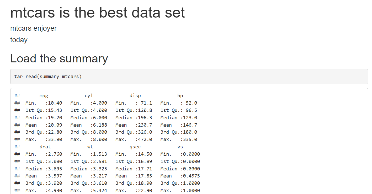
Don’t worry, we will make it look nice, but right at the end. Don’t waste time making things look good too early on. Ideally, try to get the pipeline to run on a simple example, and then keep adding features. Also, try to get as much feedback as possible on the content as early as possible from your colleagues. No point in wasting time to make something look good if what you’re writing is not at all what was expected. Let’s now get the ggplot of the data to show in the document as well.
For this, simply add:
```{r}
tar_read(plot_mtcars)
```
at the bottom of the .Rmd file. Running the pipeline again will now add the plot to the document. Before continuing, let me just remind you, again, of the usefulness of {targets} by changing the underlying data. Run the following:
write.csv(head(mtcars),
          "mtcars.csv",
          row.names = F)
and run the pipeline again. Because the data changed and every target depends on the data, the document gets entirely rebuilt. I hope that you see why this is really great: in case you need to build weekly, daily, heck, even hourly reports, by using {targets} the updated report can now get built automatically, and the targets that are not impacted by these recurrent updates will not need to be recomputed. Restore the data by running:
write.csv(mtcars,
          "mtcars.csv",
          row.names = F)
and rebuild the document by running the pipeline.
Now that the pipeline runs well, we can work a little on the document itself, by transforming the output into a nice looking table using {flextable}. But there is an issue however: the output of summary() on a data.frame object is not a data.frame, but a table and flextable::flextable() expects a data.frame. So if you call flextable::flextable() on the output of summary(), you’ll get an error message. Instead, we need a replacement for summary() that outputs a data.frame. This replacement is skimr::skim(); let’s go back to our pipeline and change the call to summary() to skim() (after adding the {skimr} to the list of loaded packages, as well as {flextable}):
library(targets)
library(tarchetypes)

tar_option_set(packages = c(
                 "dplyr",
                 "flextable",
                 "ggplot2",
                 "skimr"
                 )
               )

list(
  tar_target(
    path_data_mtcars,
    "mtcars.csv",
    format = "file"
  ),
  tar_target(
    data_mtcars,
    read.csv(path_data_mtcars)
  ),
  tar_target(
    summary_mtcars,
    skim(data_mtcars)
  ),
  tar_target(
    clean_mtcars,
    mutate(data_mtcars,
           am = as.character(am))
  ),
  tar_target(
    plot_mtcars,
    {ggplot(clean_mtcars) +
       geom_point(aes(y = mpg,
                      x = hp,
                      shape = am))}
  ),
  tar_render(
    my_doc,
    "my_document.Rmd"
  )
)
In the .Rmd file, we can now pass the output of tar_read(summary_mtcars) to flextable():
## Load the summary

```{r}
tar_read(summary_mtcars) %>%
  flextable()
```
If you run the pipeline and look at the output now, you’ll see a nice table with a lot of summary statistics. Since the output of skim() is a data.frame, you can only keep the stats you want by dplyr::select()ing the columns you need:
## Load the summary

```{r}
tar_read(summary_mtcars) %>%
  select(Variable = skim_variable,
         Mean = numeric.mean,
         SD = numeric.sd,
         Histogram = numeric.hist) %>%
  flextable()
```
If you want to hide all the R code in the output document, simply use knitr::opts_chunk$set(echo = F) in the source .Rmd file, or if you want to hide the code from individual chunks use echo = FALSE in the chunks header. Here is what the final source code of the .Rmd could look like:
---
title: "mtcars is the best data set"
author: "mtcars enjoyer"
date: today
---

```{r, include = FALSE}
# Hides all source code
knitr::opts_chunk$set(echo = F)
```


## Load the summary statistics

I really like to see the distribution of the
variables as a cell of a table:

```{r}
tar_read(summary_mtcars) %>%
  select(Variable = skim_variable,
         Mean = numeric.mean,
         SD = numeric.sd,
         Histogram = numeric.hist) %>%
  flextable() %>%
  set_caption("Summary statistics for mtcars")
```


## Graphics

The plot below is really nice, just look at it:

```{r, fig.cap = "Scatterplot of `mpg` and `hp` by type of transmission"}
tar_read(plot_mtcars) +
  theme_minimal() +
  theme(legend.position = "bottom")
```
As you can see, once I’ve used tar_read(), I get back the object just as if I had generated it from within the .Rmd source file, and can simply add stuff to it (like changing the theme of the ggplot). Once you’re happy with the contents, you can add output: word_document to the header of the document (just below date: today for example) to generate a Word document.
Let me reiterate the advantages of using {targets} to compile RMarkdown documents: because the computation of all the objects is handled by {targets}, compiling the document itself is very quick. All that needs to happen is loading pre-computed targets. This also means that you benefit from all the other advantages of using {targets}: only the outdated targets get recomputed, and the computation of the targets can happen in parallel. Without {targets}, compiling the RMarkdown document would always recompute all the objects, and all the objects’ recomputation would happen sequentially.
13.8 Rewriting our project as a pipeline and {renv} redux
It is now time to return our little project into a full-fledged reproducible pipeline. For this, we’re going back to our project’s folder and specifically to the fusen branch. This is the branch where we used {fusen} to turn our .Rmd into a package. This package contains the functions that we need to update the data. But remember, we wrote the analysis in another .Rmd file that we did not inflate, analyse_data.Rmd. We are now going to write a {targets} pipeline that will make use of the inflated package and compute all the targets required for the analysis. The first step is to create a new branch, but you could also create an entirely new repository if you want. It’s up to you. If you create a new branch, start from the rmd branch, since this will provide a nice starting point.
#switch to the rmd branch
owner@localhost ➤ git checkout rmd

#create and switch to the new branch called pipeline
owner@localhost ➤ git checkout -b pipeline
If you start with a fresh repository, you can grab the analyse_data.Rmd from here3.
First order of business, let’s delete save_data.Rmd (unless you started with an empty repo). We don’t need that file anymore, since everything is now available in the package we developed:
owner@localhost ➤ rm save_data.RmdLet’s now start an R session in that folder and install our {housing} package. Whether you followed along and developed the package, or skipped the previous parts and didn’t develop the package by following along, install it from my Github repository. This ensures that you have exactly the same version as me. Run the following line:
remotes::install_github("rap4all/housing@fusen",
                        ref = "1c86095")
This will install the package from my Github repository, and very specifically the version from the fusen branch at commit 1c86095 (you may need to install the {remotes} package first). Now that the package is installed, we can start building the pipeline. In the same R session, call tar_script() which will give us a nice template _targets.R file:
targets::tar_script()You should at most have three files: README.md, _targets.R and analyse_data.Rmd (unless you started with an empty repo, in which case you don’t have the README.md file). We will now change analyse_data.Rmd, to load pre-computed targets, instead of computing them inside the analyse_data.Rmd at compilation time.
First, we need to load the data. The two datasets we use are now part of the package, so we can simply load them using data(commune_level_data) and data(country_level_data). But remember, {targets} only loves pure functions, and data() is not pure! Let’s see what happens when you call data(mtcars). If you’re using RStudio, this is really visible: in a fresh session, calling data(mtcars) shows the following in the Environment pane:
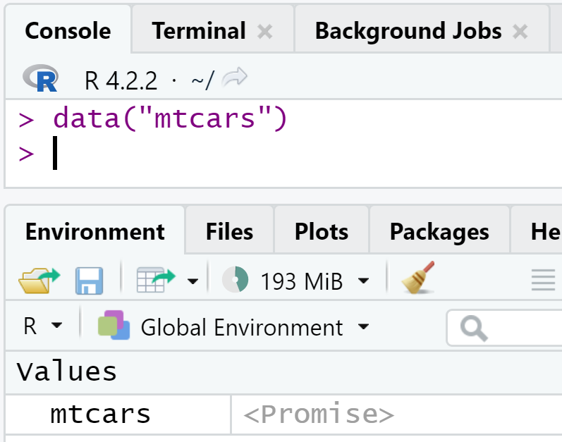
At this stage, mtcars is only a promise. It’s only if you need to interact with mtcars that the promise becomes a data.frame. So data() returns a promise, does this mean that we can save that into a variable? If you try the following:
x <- data(mtcars)And check out x, you will see that x contains the string "mtcars" and is of class character! So data() returns a promise by saving it directly to the global environment (this is a side-effect) but it returns a string. Because {targets} needs pure functions, if we write:
tar_target(
  target_mtcars,
  data(mtcars)
)
the target_mtcars target will be equal to the "mtcars" character string. This might be confusing, but just remember: a target must return something, and functions with side-effects don’t always return something, or not the thing we want. Also remember the example on plotting with plot(), which does not return an object. It’s actually the same issue here.
So to solve this, we need a pure function that returns the data.frame. This means that it first needs to load the data, which results in a promise (which gets loaded into the environment directly), and then evaluate that promise. The function to achieve this is as follows:
read_data <- function(data_name, package_name){

  temp <- new.env(parent = emptyenv())

  data(list = data_name,
       package = package_name,
       envir = temp)

  get(data_name, envir = temp)
}
This function takes data_name and package_name as arguments, both strings.
Then, I used data() but with two arguments: list = and package =. list = is needed because we pass data_name as a string. If we did something like data(data_name) instead, hoping that data_name would get replaced by its bound value ("commune_level_data") it would result in an error. This is because data() would be looking for a data set literally called data_name instead of replacing data_name by its bound value. The second argument, package = simply states that we’re looking for that dataset in the {housing} package and uses the bound value of package_name. Now comes the envir = argument. This argument tells data() where to load the data set. By default, data() loads the data in the global environment. But remember, we want our function to be pure, meaning, it should only return the data object and not load anything into the global environment! So that’s where the temporary environment created in the first line of the body of the function comes into play. What happens is that the function loads the data object into this temporary environment, which is different from the global environment. Once we’re done, we can simply discard this environment, and so our global environment stays clean.
The final step is using get(). Remember that once the line data(list = data_name...) has run, all we have is a promise. So if we stop there, the target would simply hold the character "commune_level_data". In order to turn that promise into the data frame, we use get(). We’ve already encountered this function in Chapter 7. get() searches an object by name, and returns it. So in the line get(data_name), data_name gets first replaced by its bound value, so get("commune_level_data") and hence we get the dataset back. Also, get() looks for that name in the temporary environment that was set up. This way, there is literally no interaction with the global environment, so that function is pure: it always returns the same output for the same input, and does not pollute, in any way, the global environment. After that function is done running, the temporary environment is discarded.
This seems overly complicated, but it’s all a consequence of {targets} needing pure functions that actually return something to work well. Unfortunately some of R’s default functions are not pure, so we need this kind of workaround. However, all of this work is not in vain! By forcing us to use pure functions, {targets} contributes to the general quality and safety of our pipeline. Once our pipeline is done running, the global environment will stay clean. Having stuff pollute the global environment can cause interactions with subsequent runs of the pipeline.
Let’s continue the pipeline: here is what it will ultimately look like:
library(targets)
library(tarchetypes)

tar_option_set(packages = "housing")

source("functions/read_data.R")

list(
  tar_target(
    commune_level_data,
    read_data("commune_level_data",
              "housing")
  ),

  tar_target(
    country_level_data,
    read_data("country_level_data",
              "housing")
  ),

  tar_target(
    commune_data,
    get_laspeyeres(commune_level_data)
  ),

  tar_target(
    country_data,
    get_laspeyeres(country_level_data)
  ),

  tar_target(
    communes,
    c("Luxembourg",
      "Esch-sur-Alzette",
      "Mamer",
      "Schengen",
      "Wincrange")
  ),

  tar_render(
    analyse_data,
    "analyse_data.Rmd"
  )

)
And here is what analyse_data.Rmd now looks like:
---
title: "Nominal house prices data in Luxembourg"
author: "Bruno Rodrigues"
date: "`r Sys.Date()`"
---

Let’s load the datasets (the Laspeyeres price index is already computed):

```{r}
tar_load(commune_data)
tar_load(country_data)
```

We are going to create a plot for 5 communes and compare the
price evolution in the communes to the national price evolution.
Let’s first load the communes:

```{r}
tar_load(communes)
```

```{r, results = "asis"}
res <- lapply(communes, function(x){

  knitr::knit_child(text = c(

    '\n',
    '## Plot for commune: `r x`',
    '\n',
    '```{r, echo = F}',
    'print(make_plot(country_data, commune_data, x))',
    '```'

     ),
     envir = environment(),
     quiet = TRUE)

})

cat(unlist(res), sep = "\n")

```
As you can see, the data gets loaded by using tar_load() which loads the two pre-computed data sets. The end portion of the document looks fairly similar to what we had before turning our analysis into a package and then a pipeline. We use a child document to generate as many sections as required automatically (remember, Don’t Repeat Yourself!). Try to change something in the pipeline, for example remove some communes from the communes object, and rerun the whole pipeline using tar_make().
We are now done with this introduction to {targets}: we have turned our analysis into a pipeline, and now we need to ensure that the outputs it produces are reproducible. So the first step is to use {renv}; but as already discussed, this will not be enough, but it is essential that you do it! So let’s initialize {renv}:
renv::init()This will create an renv.lock file with all the dependencies of the pipeline listed. Very importantly, our Github package also gets listed:
"housing": {
  "Package": "housing",
  "Version": "0.1",
  "Source": "GitHub",
  "RemoteType": "github",
  "RemoteHost": "api.github.com",
  "RemoteRepo": "housing",
  "RemoteUsername": "rap4all",
  "RemoteRef": "fusen",
  "RemoteSha": "1c860959310b80e67c41f7bbdc3e84cef00df18e",
  "Hash": "859672476501daeea9b719b9218165f1",
  "Requirements": [
    "dplyr",
    "ggplot2",
    "janitor",
    "purrr",
    "readxl",
    "rlang",
    "rvest",
    "stringr",
    "tidyr"
  ]
},
If you look at the fields titled RemoteSha and RemoteRef you should recognize the commit hash and repository that were used to install the package:
"RemoteRef": "fusen",
"RemoteSha": "1c860959310b80e67c41f7bbdc3e84cef00df18e",
This means that if someone wants to re-run our project, by running renv::restore() the correct version of the package will get installed! To finish things, we should edit the Readme.md file and add instructions on how to re-run the project. This is what the Readme.md file could look like:
# How to run

- Clone the repository: `git clone git@github.com:rap4all/housing.git`
- Switch to the `pipeline` branch: `git checkout pipeline`
- Start an R session in the folder and run `renv::restore()`
   to install the project’s dependencies.
- Run the pipeline with `targets::tar_make()`.
- Checkout `analyse_data.html` for the output.
If you followed along, don’t forget to change the url of the repository to your own in the first bullet point of the Readme.
13.9 Some little tips before concluding
In this section I’ll be showing you some other useful functions included in the {targets} package that I think you should know!
13.9.1 Load every target at once
It is possible to load every target included in the cache at once using tar_load_everything(). But be careful, if your pipeline builds many targets, this can take some time!
13.9.2 Get metadata information on your pipeline
tar_meta() will return a data frame with some information about the pipeline. I find it quite useful after running the pipeline, and it turns out that some warnings or errors were raised. This is how this data frame looks like:
targets::tar_meta()# A tibble: 11 × 18
name type data command depend [...]
<chr> <chr> <chr> <chr> <chr> [...]
1 analyse_d… stem c251… 995812… 3233e… [...]
2 commune_d… stem 024d… 85c2ab… ec7f2… [...]
3 commune_l… stem fb07… f48470… ce0d8… [...]
4 commune_l… stem fb07… 2549df… 15e48… [...]
5 communes stem b097… be3c56… a3dad… [...]
6 country_d… stem ae21… 9dc7a6… 1d321… [...]There are more columns than those I’m showing, of great interest are the columns warnings and error. In the example below, I have changed the code to read_data(), and now it raises a warning:
targets::tar_make()• start target commune_level_data
• built target commune_level_data [0.61 seconds]
• start target country_level_data
• built target country_level_data [0.02 seconds]
✔ skip target communes
✔ skip target commune_data
✔ skip target country_data
✔ skip target analyse_data
• end pipeline [0.75 seconds]
Warning messages:
1: this is a warning
2: this is a warning
3: 2 targets produced warnings. Run tar_meta(fields = warnings,
complete_only = TRUE) for the messages.
> Because warnings were raised, the pipeline raises another warning telling you to run tar_meta(fields = warnings, complete_only = TRUE) so let’s do it:
tar_meta(fields = warnings, complete_only = TRUE)This code returns a data frame with the name of the targets that produced the warning, alongside the warning.
# A tibble: 2 × 2
  name               warnings
  <chr>              <chr>
1 commune_level_data this is a warning
2 country_level_data this is a warning
So now you can better see what is going on.
13.9.3 Make a target (or the whole pipeline) outdated
With tar_invalidate() you can make a target outdated, so that when you rerun the pipeline, it gets re-computed (alongside every target that depends on it). This can sometimes be useful to make sure that everything is running correctly. Try running tar_invalidate("communes") and see what happens. It is also possible to complete nuke the whole pipeline and rerun it from scratch using tar_destroy(). You’ll get asked to confirm if that’s what you want to do, and if yes, reruning the pipeline after that will start from scratch.
13.9.4 Customize the network’s visualisation
By calling visNetwork::visNetworkEditor(tar_visnetwork()), a Shiny app gets started that lets you customize the look of your pipeline’s network. You can play around with the options and see the effect they have on the look of the network. It is also possible to generate R code that you can then paste into a script to consistently generate the same look.
13.9.5 Use targets from one pipeline in another project
If you need to load some targets inside another project (for example, because you need to reference an older study), you can do so easily with {withr}:
withr::with_dir(
  "path/to/root/of/project",
  targets::tar_load(target_name))
13.9.6 Understanding this cryptic error message
Sometimes, when you try to run the pipeline, you get the following error message:
Error:
! Error running targets::tar_make()
  Target errors: targets::tar_meta(fields = error, complete_only = TRUE)
  Tips: https://books.ropensci.org/targets/debugging.html
  Last error: argument 9 is empty
The last line is what interests us here: “Last error: argument 9 is empty”. It is not clear which target is raising this error: that’s because it’s not a target that is raising this error, but the pipeline itself! Remember that the pipeline is nothing but a list of targets. If your last target ends with a , character, list() is expecting another element. But because there’s none, this error gets raised. Type list(1,2,) in the console and you will get the same error message. Simply check your last target, there is a , in there that you should remove!
13.10 Conclusion
I hope to have convinced you that you need to add build automation tools to your toolbox. {targets} is a fantastic package, because it takes care of something incredibly tedious for you. By using {targets} you don’t have to remember which objects you need to recompute when you need to change code. You don’t need to rewrite your code to make it run in parallel. And by using {renv}, other users can run your pipeline in a couple of lines and reproduce the results.
In the next chapter, we will be going deeper in the iceberg of reproducibility still.