install.packages("rmarkdown")7 Literate programming
You now know about version control, how to collaborate using Github.com and functional programming. By only learning about this, you have already made some massive steps towards making your projects reproducible. Especially by using Git and Github. Even if you’re using private repos and work in the private sector, by using version control, you ensure that reusing this code for future projects is much easier. Auditing is greatly simplified as well.
But this book is still far from over. Let’s think about our project up until now. We have downloaded some data, and wrote code to analyse it. Fair enough. But usually, we don’t really stop there. We now need to write a report, or maybe a Powerpoint presentation. If you’re a researcher, you still need to write a paper, just getting the results is not enough, and if you work in the private sector, you also need to present the results of your analysis to management.
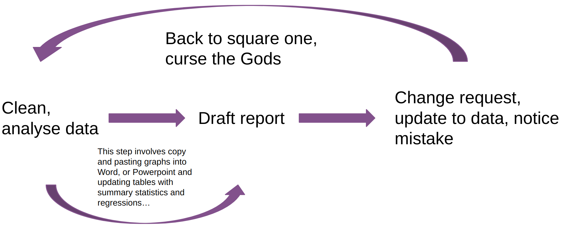
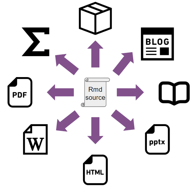
The problem is that writing code, getting some results, and putting these results into a document (it doesn’t matter what kind) is often very tedious. The picture above illustrates this cursed report drafting loop. Get some results, copy and paste images into Word or Powerpoint, get a change request, or notice a mistake, and start from scratch again. If you’re using LaTeX it’ll be easier for pictures, but you’ll still need to update tables by hand each time you need to touch your analysis code.
Worse, what if you start with a Word or LaTeX document, but then get asked to make a Powerpoint presentation as well? Then you need to copy and paste everything again, but this time into Powerpoint… and if you get a change request after you’re done and need to start over, you might seriously consider raising goats instead of dealing with this again.
But if we can make the loop look like this instead:
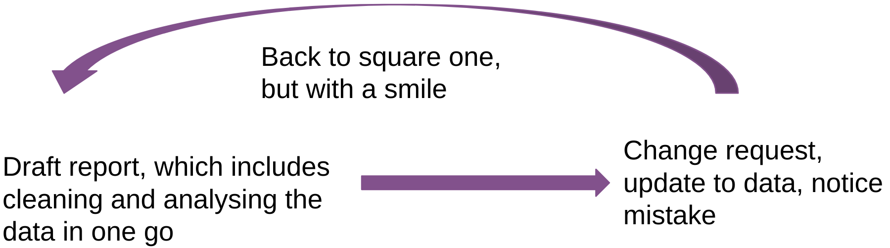
Basically, everything from cleaning, analysing and drafting is done in one single step? Well, this is what literate programming enables you to do. And even if you get asked to make a Powerpoint presentation, you can start from the same source code as the original report, and remove everything that you don’t need and compile to a Powerpoint (or Beamer) presentation.
7.1 A quick history of literate programming
In literate programming, authors mix code and prose, which makes the output of their programs not just a series of tables, or graphs or predictions, but a complete report that contains the results of the analysis directly embedded into it. Scripts written using literate programming are also very easy to compile, or render, into a variety of document formats like html, docx, pdf or even pptx. R supports several frameworks for literate programming: Sweave, knitr and Quarto.
Sweave was the first tool available to R (and S) users, and allowed the mixing of R and LaTeX code to create a document. Friedrich Leisch developed Sweave in 2002 and described it in his 2002 paper (Leisch 2002). As Leisch argues, the traditional way of writing a report as part of a statistical data analysis project uses two separate steps: running the analysis using some software, and then copy and pasting the results into a word processing tool (as illustrated above). To really drive that point home: the problem with this approach is that much time is wasted copy and pasting things, so experimenting with different layouts or data analysis techniques is very time-consuming. Copy and paste mistakes will also happen (it’s not a question of if, but when) and updating reports (for example, when new data comes in) means that someone will have, again, to copy and paste the updated results into a new document.
Sweave makes it possible to embed the analysis in the final document itself, by providing a way to mix LaTeX and R code which gets executed whenever the final, output document gets compiled. This gives practitioners considerable time savings because it eliminates the copy and pasting of results from R outputs into a document.
The snippet below shows the example from Leisch’s paper:
\documentclass[a4paper]{article}

\begin{document}

In this example we embed parts of the examples from the
\texttt{kruskal.test} help page into a LaTeX document:

<<>>=
data (airquality)
kruskal.test(Ozone ~ Month, data = airquality)
@

which shows that the location parameter of the Ozone
distribution varies significantly from month to month.
Finally we include a boxplot of the data:

\begin{center}
<<fig=TRUE,echo=FALSE>>=
boxplot(Ozone ~ Month, data = airquality)
@
\end{center}

\end{document}
Even if you’ve never seen a LaTeX source file, you should be able to figure out what’s going on. The first line states what type of document we’re writing. Then comes \begin{document} which tells the compiler where the document starts. Then comes the content. You can see that it’s a mixture of plain English with R code defined inside chunks starting with <<>>= and ending with @. Finally, the document ends with \end{document}. Getting a human-readable PDF from this source is a two-step process: first, this source gets converted into a .tex file and then this .tex file into a PDF. Sweave is included with every R installation since version 1.5.0, and still works to this day. For example, we can test that our Sweave installation works just fine by compiling the example above. This is what the final output looks like:
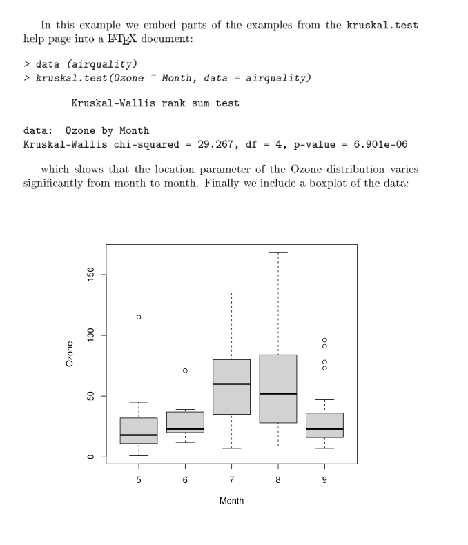
Let me just state that the fact that it is still possible to compile this example more than 20 years later is an incredible testament to how mature and stable this software is (both R, Sweave, and LaTeX). But as impressive as this is, LaTeX has a steep learning curve, and Leisch even advocated the use of the Emacs text editor to edit Sweave files, which also has a very steep learning curve (but this is entirely optional; for example, I’ve edited and compiled the example on the RStudio IDE).
The next generation of literate programming tools was provided by a package called {knitr} in 2012. From the perspective of the user, the biggest change from Sweave is that {knitr} is able to use many different formats as source files. The one that became very likely the most widely used format is a flavour of the Markdown markup language, R Markdown (Rmd). But this is not the only difference with Sweave:{knitr} can also run code chunks for other languages, such as Python, Perl, Awk, Haskell, bash and more (Xie 2014). Since version 1.18, {knitr} uses the {reticulate} package to provide a Python engine for the Rmd format.
To illustrate the Rmd format, let’s rewrite the example from Leisch’s Sweave paper into it:
---
output: pdf_document
---

In this example we embed parts of the examples from the
\texttt{kruskal.test} help page into a LaTeX document:

```{r}
data (airquality)
kruskal.test(Ozone ~ Month, data = airquality)
```


which shows that the location parameter of the Ozone
distribution varies significantly from month to month.
Finally we include a boxplot of the data:

```{r, echo = FALSE}
boxplot(Ozone ~ Month, data = airquality)
```
This is what the output looks like:
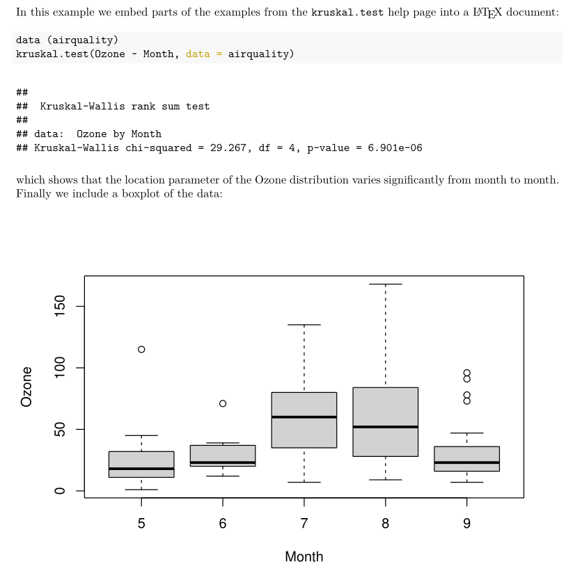
Just like in a Sweave document, an Rmd source file also has a header in which authors can define a number of general options. Here I’ve only specified that I wanted a pdf document as an output file. I then copy and pasted the contents from the Sweave source, but changed the chunk delimiters from <<>>= and @ to ```{r} to start an R chunk and ``` to end it. Remember; we need to specify the engine in the chunk because {knitr} supports many engines. For example, it is possible to run a bash command by adding this chunk to the source:
---
output: pdf_document
---

In this example we embed parts of the examples from the
\texttt{kruskal.test} help page into a LaTeX document:

```{r}
data (airquality)
kruskal.test(Ozone ~ Month, data = airquality)
```

which shows that the location parameter of the Ozone
distribution varies significantly from month to month.
Finally we include a boxplot of the data:

```{r, echo = FALSE}
boxplot(Ozone ~ Month, data = airquality)
```

```{bash}
pwd
```
(bash’s pwd command shows the current working directory). You may have noticed that I’ve also kept two LaTeX commands in the source Rmd, \texttt{} and LaTeX. This is because Rmd files get first converted into LaTeX files and then into a PDF. If you’re using RStudio, this document can be compiled by clicking a button or using a keyboard shortcut, but you can also use the rmarkdown::render() function. This function does two things transparently: it first converts the Rmd file into a source LaTeX file, and then converts it into a PDF. It is of course possible to convert the document to a Word document as well, but in this case, LaTeX commands will be ignored. Html is another widely used output format.
If you’re a researcher and prefer working with LaTeX directly instead of having to switch to Markdown, you can either use Sweave, or use {knitr} but instead of writing your documents using the R Markdown format, you can use the Rnw format which is basically the same as Sweave, but uses {knitr} for compilation. Take a look at this example1 from the {knitr} Github repository for example.
You should know that {knitr} makes it possible to author many, many different types of documents. It is possible to write books, blogs, package documentation (and even entire packages, as we shall see later in this book), Powerpoint slides… It is extremely powerful because we can use the same general R Markdown knowledge to build many different outputs.
Finally, the latest in literate programming for R is a new tool developed by Posit, called Quarto. If you’re an R user and already know {knitr} and the Rmd format, you should be able to immediately use Quarto. So what’s the difference? In practice and for R users not much but there are some things that Quarto is able to do out of the box for which you’d need extensions with {knitr}. Quarto has some nice defaults; in fact, this book is written in Quarto’s Markdown flavour and compiled with Quarto instead of {knitr} because the default Quarto output looks nicer than the default {knitr} output. However, there may even be things that Quarto can’t do at all (at least for now) when compared to {knitr}. So why bother switching? Well, Quarto provides sane defaults and some nice features out of the box, and the cost of switching from the Rmd format to Quarto’s Qmd format is basically 0. Also, and this is probably the biggest reason to use Quarto, Quarto is not tied to R. Quarto is actually a standalone tool that needs to be installed alongside your R installation, and works completely independently. In fact, you can use Quarto without having R installed at all, as Quarto, just like {knitr} supports many engines. This means that if you’re primarily using Python, you can use Quarto to author documents that mix Python chunks and prose. Quarto also supports the Julia programming language and Observable JS, making it possible to include interactive visualisations into an Html document. Let’s take a look at how the example from Leisch’s paper looks as a Qmd (Quarto’s flavour of Markdown) file:
---
output: pdf
---

In this example we embed parts of the examples from the
\texttt{kruskal.test} help page into a LaTeX document:

```{r}
data (airquality)
kruskal.test(Ozone ~ Month, data = airquality)
```


which shows that the location parameter of the Ozone
distribution varies significantly from month to month.
Finally we include a boxplot of the data:

```{r, echo = FALSE}
boxplot(Ozone ~ Month, data = airquality)
```
(I’ve omitted the bash chunk from before, not because Quarto does not support it, but to keep close to the original example from the paper.)
As you can see, it’s exactly the same as the Rmd file from before. The only difference is in the header. In the Rmd file I specified the output format as:
---
output: pdf_document
---
whereas in the Qmd file we changed it to:
---
output: pdf
---
While Quarto is the latest option in literate programming, it is quite recent, and as such, I feel it might be better to stick with {knitr} and the Rmd format for now, so that’s what we’re going to use going forward. Also, the {knitr} and the Rmd format are here to stay, so there’s little risk in keeping using it, and anyways, as already stated, if switching to Quarto becomes a necessity, the cost of switching would be very, very low. In what follows, I won’t be focused on anything really {knitr} or Rmd specific, so should you want to use Quarto instead, you should be able to follow along without any problems at all, since the Rmd and Qmd formats have so much overlap. Also, Quarto needs to be installed separately, but to use {knitr} and RMarkdown, no specific tools are necessary.
In the next two sections, I will show you how to set up and use {knitr} as well as give you a quick overview of the R Markdown syntax. However, we will very quickly focus on the templating capabilities of {knitr}: expanding text, using child documents, and parameterised reports. These are advanced topics and not easy to tackle if you’re not comfortable with R already. Just as functions and higher-order functions like lapply() avoid having to repeat yourself, so does templating, but for literate programming. The goal is to write functions that return literal R Markdown code, so that you can loop over these functions to build entire sections of your documents. However, the learning curve for these features is quite steep, but by now, you should have noticed that this book expects a lot from you. Keep going, and you shall be handsomely rewarded.
7.2 {knitr} basics
This section will be a very small intro to {knitr}. I’m going to teach you just enough to get started writing Rmd files. Most, if not all, of what I’ll be explaining here is also applicable to the Qmd format. There are many resources out there that you can use if you want to dig deeper, for instance the R Markdown website2 from Posit, or the R Markdown: The Definitive Guide3 and R Markdown Cookbook4 eBooks. I will also not assume that you are using the RStudio IDE and give you instead the lower level commands to render documents. If you use RStudio and want to know how to use it effectively to author Rmd documents, you should take a look at this5 page. In fact, this section will basically focus on the same topics, but without RStudio.
7.2.1 Set up
The first step is to install the {knitr} and the {rmarkdown} packages. That’s easy, just type:
in an R console. Since {knitr} is required to install {rmarkdown}, it gets installed automatically. If you want to compile PDF documents, you should also have a working LaTeX distribution. You can skip this next part if you’re only interested in generating Html and Word files. For what follows in the book, we will only be rendering Html documents, so no need to install LaTeX (by the way, you don’t even need a working Word installation to compile documents to the docx format). However, if you already have a working LaTeX installation, you shouldn’t have to do anything else to generate PDF documents. If you don’t have a working LaTeX distribution, then Yihui Xie, the creator of {knitr} created an R package called {tinytex} which you can use to install a working LaTeX distribution very easily. In fact, this is the way I recommend installing LaTeX even if you’re not an R user (it is possible to use the tinytex distribution without R; it’s just that the {tinytex} R package provides many functions that makes installing and maintaining it very easy). Simply run these commands in an R console to get started:
install.packages("tinytex")
tinytex::install_tinytex()
and that’s it! If you need to install specific LaTeX packages, then refer to the Maintenance section on tinytex’s6 website. For example, to compile the example from Leisch’s article on Sweave discussed previously, the grfext LaTeX package needs to be installed (as explained by the error output in the console when I tried compiling). To install this package, you can use the tlmgr_install() function from {tinytex}:
tlmgr_install("grfext")After you’ve installed {knitr}, {rmarkdown} and, optionally, {tinytex}, simply try to compile the following document:
---
output: html_document
---

# Document title

## Section title

### Subsection title

This is **bold** text. This is *text in italics*.

My favourite programming language for statistics is ~~SAS~~ R.
save this document into a file called rmd_test.rmd using your favourite text editor. Then render it into an Html file by running the following command in the R console:
rmarkdown::render("path/to/rmd_test.rmd")This should create a file called rmd_test.html; open it with your web browser and you should see the following:
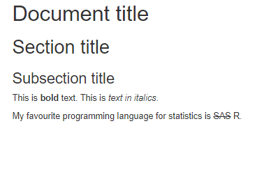
Congratulations, you just knitted your first Rmd document!
7.2.2 Markdown ultrabasics
R Markdown is a flavour of Markdown, which means that you should know some Markdown to really take full advantage of R Markdown. The example document from before should have already shown you some basics: titles, sections and subsections all start with a # and the depth level is determined by the number of #s. For bold text, simply put the words in between ** and for italics use only one *. If you want bold and italics, use ***. The original designer of Markdown did not think that underlining text was important, so there is no easy way of doing it, unfortunately. For this, you need to use a somewhat hidden feature; without going into too many technical details, the program that converts Rmd files to the final output format is called Pandoc, and it’s possible to use some of Pandoc’s features to format text. For example, for underlining:
[This is some underlined text in a R Markdown document]{.underline}This will underline the text between square brackets.7
The next step is to mix code and prose. As you’ve seen from Leisch’s canonical example, this is quite easily achieved by using R code chunks. The R Markdown example below shows various code chunks alongside some options. For example, a code chunk that uses the echo = FALSE option will not appear (but the output of the computation will):
---
title: "Document title"
output: html_document
date: "2023-01-28"
---

# R code chunks

This below is an R code chunk:

```{r}
data(mtcars)

plot(mtcars)
```


The code chunk above will appear in the final output.
The code chunk below will be hidden:

```{r, echo = FALSE}
data(iris)

plot(iris)
```


This next code chunk will not be evaluated:

```{r, eval = FALSE}
data(titanic)

str(titanic)
```


The last one below runs, but code and output from the code is
not shown in the final document. This is useful for loading
libraries and hiding startup messages:

```{r, include = FALSE}
library(dplyr)
```
If you use RStudio and create a new R Markdown file from the menu, a template R Markdown file is generated for you to fill out. The first R chunk is this one:
```{r setup, include=FALSE}
knitr::opts_chunk$set(echo = TRUE)
```
This is an R chunk named setup with the option include = FALSE (so neither the chunk itself, nor the output it produces will be shown in the compiled document). Naming chunks is optional, but we are going to make use of this later on. The code that runs in this chunk defines a global option to show the source code from all the chunks by default (which is the default behaviour). You can change TRUE to FALSE if you want to hide every code chunk instead (if you’re using Quarto, global options are set differently8).
Something else you might have noticed in the previous example, is that we’ve added some more content in the header:
---
title: "Document title"
output: html_document
date: "2023-01-28"
---
There are several other options available that you can define in the header. Later on, I will show you some more options, for example how to define a table of contents.
To finish this part on code chunks, you should know about inline code chunks. Take a look at the following example:
---
title: "Document title"
output: html_document
date: "2023-01-28"
---

# R code chunks

```{r, echo = FALSE}
data(iris)
```


The iris dataset has `r nrow(iris)` rows.
The last sentence from this example has an inline code chunk. This is quite useful, as it allows to parameterise sentences and paragraphs, and thus avoids needing to copy and paste (and we will go quite far into how to avoid copy and pasting, thanks to more advanced features we will shortly discuss).
To finish this crash course, you should know that to use footnotes you need to write the following:
This sentence has a footnote.[^1]

[^1]: This is the footnote.
or the following (which I prefer):
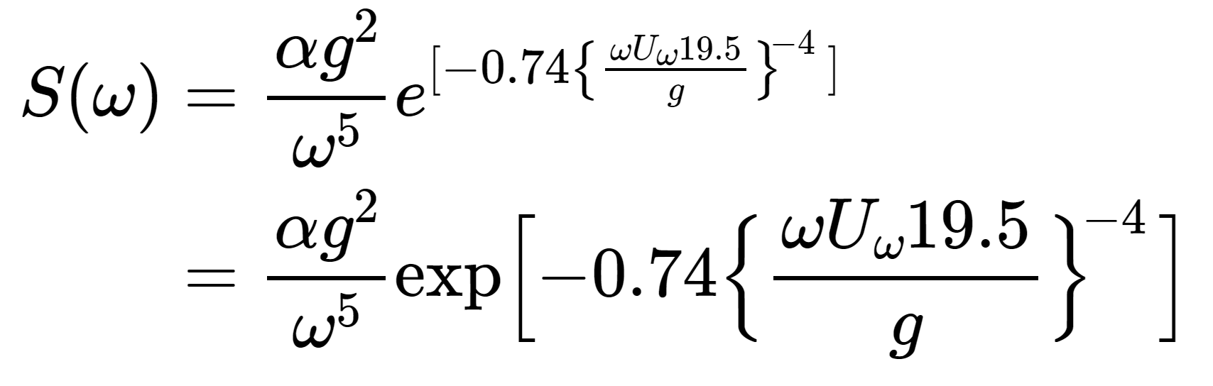
This sentence has a footnote.^[This is the footnote]and that you can write LaTeX formulas as well. For example, add the lines below into the example from before and render either a PDF or an HTML document (don’t put the LaTeX formula below inside a chunk, simply paste it as if it were normal text. This doesn’t work for Word output because Word does not support LaTeX equations):
\begin{align*}
S(\omega)
&= \frac{\alpha g^2}{\omega^5}
  e^{[ -0.74\bigl\{\frac{\omega U_\omega 19.5}{g}\bigr\}
   ^{\!-4}\,]} \\
&= \frac{\alpha g^2}{\omega^5}
\exp\Bigl[ -0.74\Bigl\{\frac{\omega U_\omega 19.5}{g}\Bigr\}
  ^{\!-4}\,\Bigr]
\end{align*}
The LaTeX code above results in this equation:
7.3 Keeping it DRY
Remember; we never, ever, want to have to repeat ourselves. Copy and pasting is forbidden. Striving for 0 copy and pasting will make our code much more robust and likely to be correct.
To keep DRY, we started by using functions, as discussed in the previous chapter, but we can go much further than that. For example, suppose that we need to write a document that has the following structure:
- A title
- A section
- A table inside this section
- Another section
- Another table inside this section
- Yet another section
- Yet another table inside this section
Is there a way to automate the creation of such a document by taking advantage of the repeating structure? Of course there is. The question is not, is it possible to do X?, but how to do X?.
7.3.1 Generating R Markdown code from code
The example below is a fully working minimal example of this. Copy it inside a document titled something like rmd_templating.Rmd and render it. You will see that the output contains more sections than defined in the source. This is because we use templating at the end. Take some time to read the document, as the text inside explains what is going on:
---
title: "Templating"
output: html_document
date: "2023-01-27"
---

```{r setup, include=FALSE}
knitr::opts_chunk$set(echo = TRUE)
```


## A function that creates tables

```{r}
create_table <- function(dataset, var){
  table(dataset[var]) |>
    knitr::kable()
}
```


The function above uses the `table()` function to create
frequency tables, and then this gets passed to the
`knitr::kable()` function that produces a good looking table
for our rendered document:

```{r}
create_table(mtcars, "am")
```


Let’s suppose that we want to generate a document that would
look like this:

- first a section title, with the name of the variable of interest
- then the table

So it would look like this:

## Frequency table for variable: "am"

```{r}
create_table(mtcars, "am")
```


We don’t want to create these sections for
every variable by hand.

Instead, we can define a function that
returns the R markdown code required to
create this. This is this function:

```{r}
return_section <- function(dataset, var){
  a <- knitr::knit_expand(text = c(
               "## Frequency table for variable: {{variable}}",
                create_table(dataset, var)),
                variable = var)
  cat(a, sep = "\n")
}
```


This new function, `return_section()` uses
`knitr::knit_expand()` to generate RMarkdown
code. Words between `{{}}` get replaced by
the provided `var` argument to the function.
So when we call `return_section("am")`,
`{{variable}}` is replaced by `"am"`. `"am"`
then gets passed down to `create_table()`
and the frequency table gets generated.
We can now generate all the section by simply
applying our function to a list of column names:

```{r, results = "asis"}
invisible(lapply(colnames(mtcars), return_section, dataset = mtcars))
```
The last function, named return_section() uses knit_expand(), which is the function that does the heavy lifting. This function returns literal R Markdown code. It returns ## Frequency table for variable: {{variable}} which creates a level 2 section title with the text Frequency table for variable: xxx where the xxx will get replaced by the variable passed to return_section(). So calling return_section(mtcars, "am") will print the following in your console:
## Frequency table for variable: am
|am | Freq|
|:--|----:|
|0  |   19|
|1  |   13|
We now simply need to find a clever way to apply this function to each variable in the mtcars dataset. For this, we are going to use lapply() which implements a for loop (you could use purrr::map() just as well for this):
invisible(lapply(colnames(mtcars),
                 return_section,
                 dataset = mtcars))
This will create, for each variable in mtcars, the same R Markdown code as above. Notice that the R Markdown chunk where the call to lapply() is has the option results = "asis". This is because the function returns literal Markdown code, and we don’t want the parser to have to parse it again. We tell the parser “don’t worry about this bit of code, it’s already good”. As you see, the call to lapply() is wrapped inside invisible(). This is because return_section() does not return anything, it just prints something to the console. No object is returned. return_section() is a function with only a side-effect: it changes something outside its scope. So if you don’t wrap the call to lapply() inside invisible(), then a bunch of NULLs will also get printed (NULLs get returned by functions that don’t return anything). To avoid this, use invisible() (and use purrr::walk() rather than purrr::map() if you want to use tidyverse packages and functions).
This is not an easy topic, so take the time to play around with the example above. Try to print another table, try to generate more complex Markdown code, remove the call to invisible() and knit the document and see what happens with the output, replace the call to lapply() with purrr::walk() or purrr::map(). Really take the time to understand what is going on.
While extremely powerful, this approach using knit_expand() only works if your template only contains text. If you need to print something more complicated in the document, you need to use child documents instead. For example, suppose that instead of a table we wanted to show a plot made using {ggplot2}. This would not work, because a ggplot object is not made of text, but is a list with many elements. The print() method for ggplot objects then does some magic and prints a plot. But if you want to show plots using knitr::knit_expand(), then the contents of the list will be shown, not the plot itself. This is where child documents come in. Child documents are exactly what you think they are: they’re smaller documents that get knitted and then embedded into the parent document. You can define anything within these child documents, and as such you can even use them to print more complex objects, like a ggplot object. Let’s go back to the example from before and make use of a child document (for ease of presentation, we will not use a separate Rmd file, but will inline the child document into the main document). Read the Rmd example below carefully, as all the steps are explained:
---
title: "Templating with child documents"
output: html_document
date: "2023-01-27"
---

```{r setup, include=FALSE}
knitr::opts_chunk$set(echo = TRUE)
library(ggplot2)
```

## A function that creates ggplots

```{r}
create_plot <- function(dataset, aesthetic){

  ggplot(dataset) +
    geom_point(aesthetic)

}
```

The function above takes a dataset and an aesthetic
made using `ggplot2::aes()` to create a plot:

```{r}
create_plot(mtcars, aes(y = mpg, x = hp))
```

Let’s suppose that we want to generate a document
that would look like this:

- first a section title, with the dataset used;
- then a plot

So it would look like this:

## Dataset used: "mtcars"

```{r}
create_plot(mtcars, aes(y = mpg, x = hp))
```

We don’t want to create these sections for every
aesthetic by hand.

Instead, we can make use of a child document that
gets knitted separately and then embedded in the
parent document. The chunk below makes use of this trick:

```{r, results = "asis"}

x <- list(aes(y = mpg, x = hp),
          aes(y = mpg, x = hp, size = am))

res <- lapply(x,
              function(dataset, x){

  knitr::knit_child(text = c(

    '\n',
    '## Dataset used: `r deparse(substitute(dataset))`',
    '\n',
    '```{r, echo = F}',
    'print(create_plot(dataset, x))',
    '```'

     ),
     envir = environment(),
     quiet = TRUE)

}, dataset = mtcars)


cat(unlist(res), sep = "\n")
```

The child document is the `text` argument to the
`knit_child()` function. `text` is literal R Markdown
code: we define a level 2 header, and then an R chunk.
This child document gets knitted, so we need to specify
the environment in which it should get knitted. This means
that the child document will get knitted in the same
environment as the parent document (our current global
environment). This way, every package that gets loaded
and every function or variable that got defined in the
parent document will also be available to the child document.

To get the dataset name as a string, we use the
`deparse(substitute(dataset))` trick; this substitutes
"dataset" by its bound value, so `mtcars`. But `mtcars` is
an expression and we don’t want it to get evaluated, or the
contents of the entire dataset would be used in the title
of the section. So we use `deparse()` which turns unevaluated
expressions into strings.

We then use `lapply()` to loop over two aesthetics with an
anonymous function that encapsulates the child document. So we
get two child documents that get knitted, one per aesthetic.
This gets saved into variable `res`. This is thus a list of
knitted Markdown.

Finally, we need unlist `res` to actually merge the Markdown
code from the child documents into the parent document.Here again, take some time to play with the above example. Change the child document, try to print other types of output, really take your time to understand this. To know more about child documents, take a look at this section11 of the R Markdown Cookbook (Xie, Dervieux, and Riederer 2020).
By the way, if you wish to add a table of contents to your document, change the header to this:
---
title: "Templating with child documents and TOC"
output:
  html_document:
    toc: true
    toc_float: true
date: "2023-01-27"
---
7.3.2 Tables in R Markdown documents
Getting tables right in Rmd documents is not always an easy task. There are several packages specifically made just for this task, and the package that I recommend tick the following two important boxes:
- Work the same way regardless of output format (Word, PDF or Html);
- Work for any type of table: summary tables, regression tables, two-way tables, etc.
Let’s start with the simplest type of table, which would be a table that simply shows some rows of data. {knitr} comes with the kable() function, but this function generates a very plain looking output. For something publication-worthy, we recommend the {flextable} package, developed by Gohel and Skintzos (2023):
library(flextable)

my_table <- head(mtcars)

flextable(my_table) |>
  set_caption(caption = "Head of the mtcars dataset") |>
  theme_booktabs()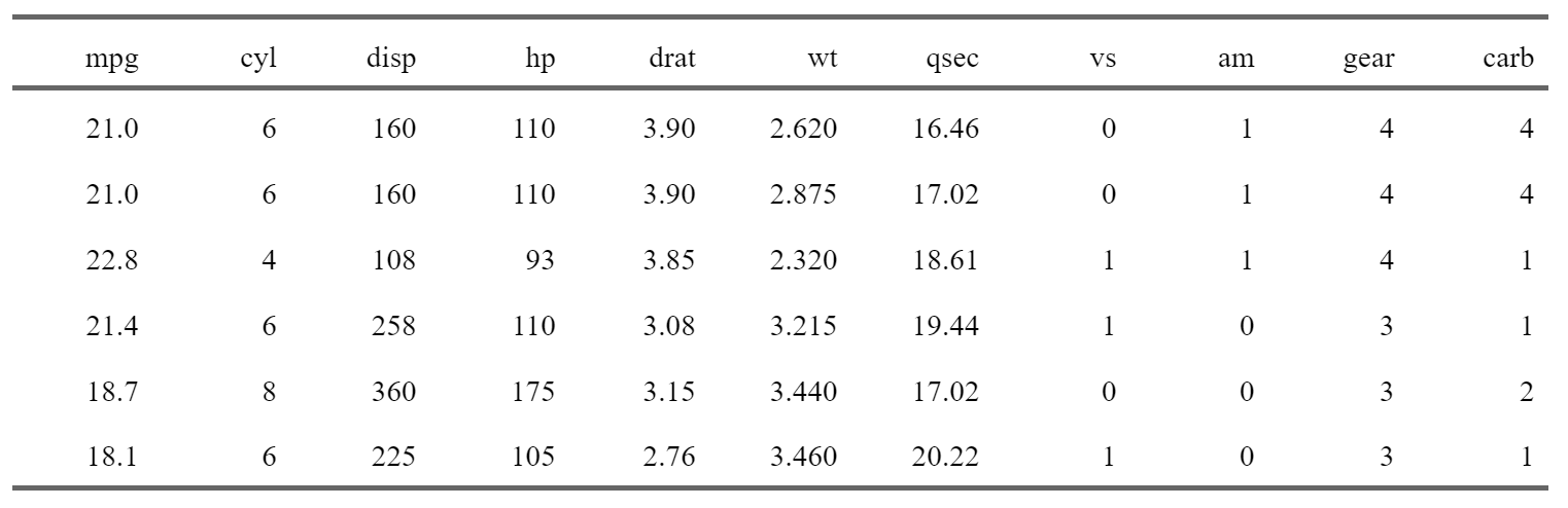
Note that the example above will work pretty much the same way for any table that you can coerce into a data frame! I won’t explain how {flextable} works, but it is very powerful, and the fact that it works for PDF, Html, Word and Powerpoint outputs is really a massive plus. If you want to learn more about {flextable}, there’s a whole, free, ebook on it12. {flextable} can create very complicated tables, so really take the time to dig in!
The next package is {modelsummary}, by Arel-Bundock (2022), and this one focuses on regression and summary tables. It is extremely powerful as well, and just like {flextable}, works for any type of output. It is very simple to get started:
library(modelsummary)

model_1 <- lm(mpg ~ hp + am, data = mtcars)
model_2 <- lm(mpg ~ hp, data = mtcars)

models <- list("Model 1" = model_1,
               "Model 2" = model_2)

modelsummary(models)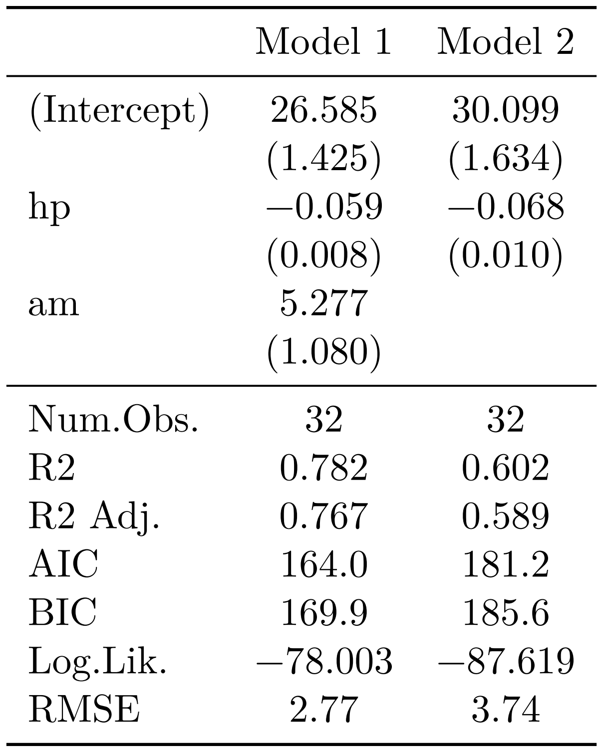
Here again, I won’t got into much detail, but recommend instead that you read the package’s website13 which has very detailed documentation.
These packages can help you keeping it DRY, so take some time to learn them.
And one last thing: if you’re a researcher, take a look at the {rticles}14 package, which provides Rmd templates to write articles for many scientific journals.
7.3.3 Parametrized reports
Templating and child documents are very powerful, but sometimes you don’t want to have one section dedicated to each unit of analysis within the same report, but rather, you want a complete separate report by unit of analysis. This is possible thanks to parameterised reports.
Let’s change the example from before, which consisted of creating one section per column of the mtcars dataset and a frequency table, and make it now one separate report for each column. The R Markdown file will look like this:
---
title: "Report for column `r params$var` of dataset `r params$dataset`"
output: html_document
date: "2023-01-27"
params:
  dataset: mtcars
  var: "am"
---

```{r setup, include=FALSE}
knitr::opts_chunk$set(echo = TRUE)
```


## Frequency table for `r params$var`

```{r, echo = F}
create_table <- function(dataset, var){

  dataset <- get(dataset)

  table(dataset[var]) |>
    knitr::kable()
}
```


The table below is for variable `r params$var` of
dataset `r params$dataset`.

```{r}
create_table(params$dataset, params$var)
```

```{r, eval = FALSE, echo = FALSE}
# Run these lines to compile the document
# Set eval and echo to FALSE, so that this does not appear
# in the output, and does not get evaluated when knitting
rmarkdown::render(
             input = "param_report_example.Rmd",
             params = list(
               dataset = "mtcars",
               var = "cyl"
             )
           )

```
Save the code above into an Rmd file titled something like param_report_example.Rmd (preferably inside its own folder). Note that at the end of the document, I wrote the lines to render this document inside a chunk that does not get shown to the reader, nor gets evaluated:
```{r, eval = F, echo = FALSE}
rmarkdown::render(
             input = "param_report_example.Rmd",
             params = list(
               dataset = "mtcars",
               var = "cyl"
             )
           )
```
You need to run these lines yourself to knit the document.
This will pass the list params with elements “mtcars” and “cyl” down to the report. Every params$dataset and params$var in the report gets replaced by “mtcars” and “cyl” respectively. Also, notice that in the header of the document, I defined default values for the params. Something else you need to be aware of, is that the function create_table() inside the report is slightly different than before. It now starts with the following line:
dataset <- get(dataset)Let’s break this down. params$dataset contains the string “mtcars”. I made the decision to pass the dataset as a string, so that I could use it in the title of the document. But then, inside the create_table() function, I have the following code:
dataset[var]dataset can’t be a string here, but needs to be a variable name, so mtcars and not "mtcars". This means that I need to convert that string into a name. get() searches an object by name, and then makes it possible to save it to a new variable called dataset. The rest of the function is then the same as before. This little difficulty can be avoided by hard-coding the dataset inside the R Markdown file, or by passing the dataset as the params$dataset and not the string, in the render function. However, if you pass down the name of the dataset as a variable instead of the dataset name as a string, then you need to covert it to a string if you want to use it in the text (so mtcars to "mtcars", using deparse(substitute(dataset)) as in child documents example).
If you instead want to create one report per variable, you could compile all the documents at once with:
```{r, eval = F, echo = F}
columns <- colnames(mtcars)

lapply(columns,
  (\(x)rmarkdown::render(
                    input = "param_report_example.Rmd",
                    output_file = paste0(
                      "param_report_example_", x, ".html"
                    ),
                    params = list(
                      dataset = "mtcars",
                      var = x
                    )
                  )
  )
)
```
By now, this should not intimidate you anymore; I use lapply() to loop over a list of column names (that I get using colnames()). Because I don’t want to overwrite the report I need to change the name of the output file. I do so by using paste0() which creates a new string that contains the variable name, so each report gets its own name. x inside the paste0() function is each element, one after the other, of the columns variable I defined first. Think of it as the i in a for loop. I then must also pass this to the params list, hence the var = x. The complete call to rmarkdown::render() is wrapped inside an anonymous function, because I need to use the argument x (which is each column defined in the columns list) in different places.
7.4 Conclusion
Before continuing, I highly recommend that you try running this yourself, and also that you try to build your own little parameterised reports. Maybe start by replacing “mtcars” by “iris” in the code to compile the reports and see what happens, and then when you’re comfortable with parameterised reports, try templating inside a parameterised report!
It is important not to succumb to the temptation of copy and pasting sections of your report, or parts of your script, instead of using these more advanced features provided by the language. It is tempting, especially under time pressure, to just copy and paste bits of code and get things done instead of writing what seems to be unnecessary code to finally achieve the same thing. The problem, however, is that in practice copy and pasting code to simply get things done will come bite you sooner rather than later. Especially when you’re still in the exploration/drafting phase of the project. It may take more time to set up, but once you’re done, it is much easier to experiment with different parameters, test the code or even re-use the code for other projects. Not only that but forcing you to actually think about how to set up your code in a way that avoids repeating yourself also helps with truly understanding the problem at hand. What part of the problem is constant and does not change? What does change? How often, and why? Can you also fix these parts or not? What if instead of five sections that I need to copy and paste, I had 50 sections? How would I handle this?
Asking yourself these questions, and solving them, will ultimately make you a better programmer.
Remember: don’t repeat yourself!
https://is.gd/Z7VS09↩︎
https://rmarkdown.rstudio.com/lesson-1.html↩︎
https://bookdown.org/yihui/rmarkdown/↩︎
https://bookdown.org/yihui/rmarkdown-cookbook/↩︎
https://rmarkdown.rstudio.com/authoring_quick_tour.html↩︎
https://yihui.org/tinytex/#maintenance↩︎
https://stackoverflow.com/a/68690065/1298051↩︎
https://quarto.org/docs/computations/execution-options.html↩︎
https://is.gd/EzdUtt↩︎
https://is.gd/aR2hyz↩︎
https://is.gd/gAqzf9↩︎
https://ardata-fr.github.io/flextable-book/index.html↩︎
https://is.gd/pjIKmV↩︎
https://pkgs.rstudio.com/rticles/articles/examples.html↩︎